Linear Arrays
•A linear array is a list of a
finite number of n
homogeneous
data elements ( that is data elements of the same type) such that
–The elements are of the arrays are
referenced respectively by an index set consisting of n
consecutive numbers
–The elements of the arrays are
stored respectively in successive
memory locations .
•The
number n
of
elements is called the length or size of the array.
•The
index set consists of the integer 1,
2, … n
•Length
or the number of data elements of the array can be obtained from the index set
by
Length
= UB – LB + 1 where UB is
the largest index called the upper
bound and LB is
the smallest index called the lower
bound of the arrays .
•Element of an array A may
be denoted by
–Subscript notation A1,
A2, , …. , An
–Parenthesis notation A(1), A(2), …. , A(n)
–Bracket notation A[1], A[2], ….. , A[n]
–
•The number K in
A[K] is called subscript or an index and A[K] is called a subscripted variable
Related post :Data Structure vs Storage Structure
Related post :Data Structure vs Storage Structure
Representation of Linear Array in Memory
•Let
LA be a
linear array in the memory of the computer
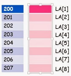
•LOC(LA[K]) = address of the element
LA[K] of the array LA
•The
element of LA
are stored in the successive memory cells
•Computer
does not need to keep track of the
address of every element of LA,
but need to track only the address of the first element of the array denoted by
Base(LA) called
the base
address of LA
•LOC(LA[K])
= Base(LA) + w(K – lower bound) where
w is
the number of words per memory cell of the array LA [w is
aka size of the data
type] .
Example 1 :
LOC(LA[K])
= Base(LA) + w(K – lower bound)
LOC(LA[6])
= 200 + 1(6 – 1) = 205
Example 2:
Find
the address for LA[16]
Each
element of the array occupy 2 byte
LOC(LA[K])
= Base(LA) + w(K – lower bound)
LOC(LA[16]) = 200 + 2(16 – 1) =230
Representation of Linear Array in Memory
•Given
any value of K,
time to calculate LOC(LA[K])
is
same
•Given
any subscript K
one can access and locate the content
of LA[K]
without scanning any other element of LA
•A
collection A
of data element is said to be index if any element of A
called Ak
can be located and processed in time that
is independent of K
Traversing Linear Arrays
•Traversing is accessing and
processing (aka visiting ) each element of the data structure exactly ones
1.Repeat
for K = Lower Bound to Upper Bound
Apply PROCESS to LA[K]
[End of Loop]
2. Exit
Insertion in array
•Insertion:
Adding an element
–Beginning
–Middle
–End
DEMO 1
Insert Ford at the
End of Array
Deletion in array
•Deletion:
Removing an element
–Beginning
–Middle
–End
Related post >>Double link list
DEMO 1
Deletion
of Wagner at the End of
Array
Insertion Algorithm
•INSERT
(LA, N , K , ITEM)
[LA is a linear array with N
elements and K is a positive integers such that K ≤ N. This algorithm insert an
element ITEM into the Kth
position in LA ]
1. [Initialize
Counter] Set J := N
2. Repeat
Steps 3 and 4 while J ≥ K
3. [Move
the Jth
element downward ] Set LA[J + 1] :=
LA[J]
4. [Decrease
Counter] Set J := J -1
5 [Insert
Element] Set LA[K] := ITEM
6. [Reset
N] Set N := N +1;
7. Exit
Deletion Algorithm
•DELETE
(LA, N , K , ITEM)
[LA is a linear array with N
elements and K is a positive integers such that K ≤ N. This algorithm deletes Kth
element from LA ]
1. Set
ITEM := LA[K]
2. Repeat
for J = K to N -1:
[Move the J + 1st
element upward] Set LA[J] := LA[J + 1]
3. [Reset
the number N of elements] Set N := N - 1;
4. Exit


No comments:
Post a Comment
THANKS FOR UR GREAT COMMENT